Tutorial

The following script is used to fit micribiome count data and covariate data to the integrative Bayesian zero-inflated negative binomial hierarchical mixture model proposed in the manuscript

Before running the following code, please first load micribiome count data and covariate data. The necessary inputs should be

a n-by-p count matrix Y, where n is the number of samples and p is the number of taxa(feature)
a n-by-R covaritae matrix X, where R is the number of covariates
a n-dimensional vector z, indicating group allocation for n samples

You also need to install Rcpp, RcppArmadillo and pROC packages.

Load functions & data matrices

library(IntegrativeBayes)
#> Loading required package: pROC
#> Warning: package 'pROC' was built under R version 3.5.2
#> Type 'citation("pROC")' for a citation.
#> 
#> Attaching package: 'pROC'
#> The following objects are masked from 'package:stats':
#> 
#>     cov, smooth, var
load(system.file("extdata/Example_data.Rdata", package = "IntegrativeBayes"));

Preprocessing

# keep the features that have at least 2 observed counts for both groups:
Y.input = Y.filter(Y.mat, zvec = z.vec, min.number = 2)[[2]]
#> 300 out of 300 features are kept.
# estimate the size factor s from the count matrix Y:
s.input = sizefactor.estimator(Y.mat)

Get true label for later visualization

feature.remain = which(Y.filter(Y.mat, zvec = z.vec, min.number = 2)[[1]] == 1)
#> 300 out of 300 features are kept.
gamma.vec = gamma.vec[feature.remain]
delta.mat = delta.mat[,feature.remain]

Implement MCMC algorithm

S.iter = 10000
burn.in = 0.5
mu0.start = 10
res = zinb_w_cov(Y_mat = Y.input,
                 z_vec = z.vec, 
                 s_vec = s.input,
                 X_mat = X.mat,
                 S = S.iter, burn_rate = burn.in,
                 mu0_mean = mu0.start)
#> 0% has been done
#> 10% has been done
#> 20% has been done
#> 30% has been done
#> 40% has been done
#> 50% has been done
#> 60% has been done
#> 70% has been done
#> 80% has been done
#> 90% has been done

The MCMC outputs are stored in res: $mu0 est: posterior mean(after burn-in) for the vector mu(0j) $phi est: posterior mean(after burn-in) for the dispersion parameter vector $beta est: posterior mean(after burn-in) for the Beta matrix $gamma PPI: PPI for all gamma(j) after burn-in $delta PPI: PPI for all delta(rj) fter burn-in $R PPI: PPI for all r(ij) after burn-in $gamma sum: sum of all gamma(j) for all iterations $mukj full: MCMC draws for mu(kj) after burn-in $mu0 full: MCMC draws for mu(0j) after burn-in $beta full: MCMC draws for beta(rj) after burn-in

Visualizing the results for two variable selection processes

Variable selection for discriminating features

The stem-plot showed the selected features passing Bayesian FDR threshold.

gamma_VS(res$gamma_PPI, gamma.true = gamma.vec)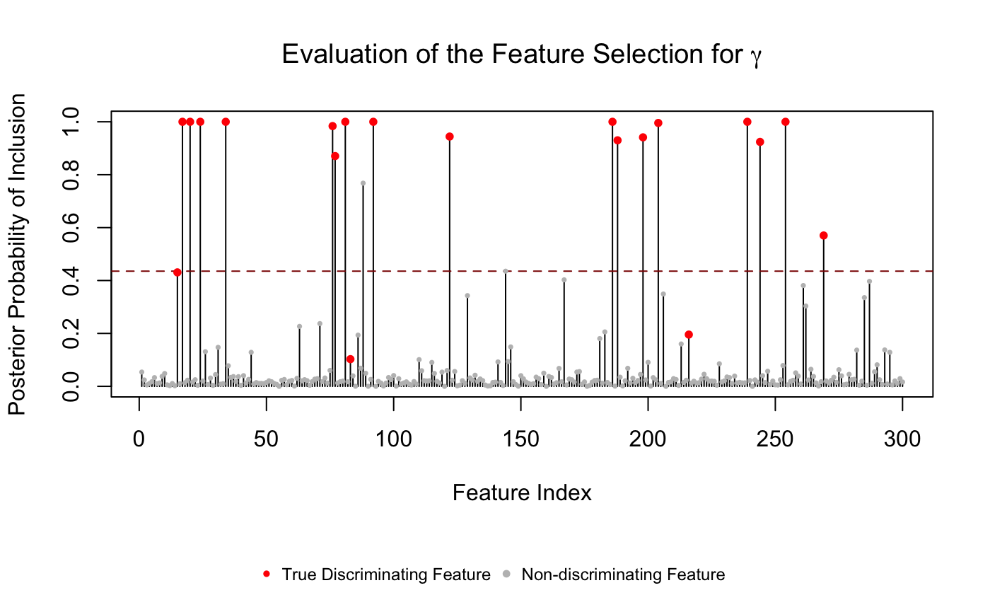

par(mar=c(5.1, 4.1, 4.1, 2.1))

Variable selection for significant feature-covariate association

The ROC plot was used to benchmark the performance of detecting microbiome-covariate associations.

delta_ROC(as.vector(res$delta_PPI), as.vector(abs(delta.mat)))
#> Setting levels: control = 0, case = 1
#> Setting direction: controls < cases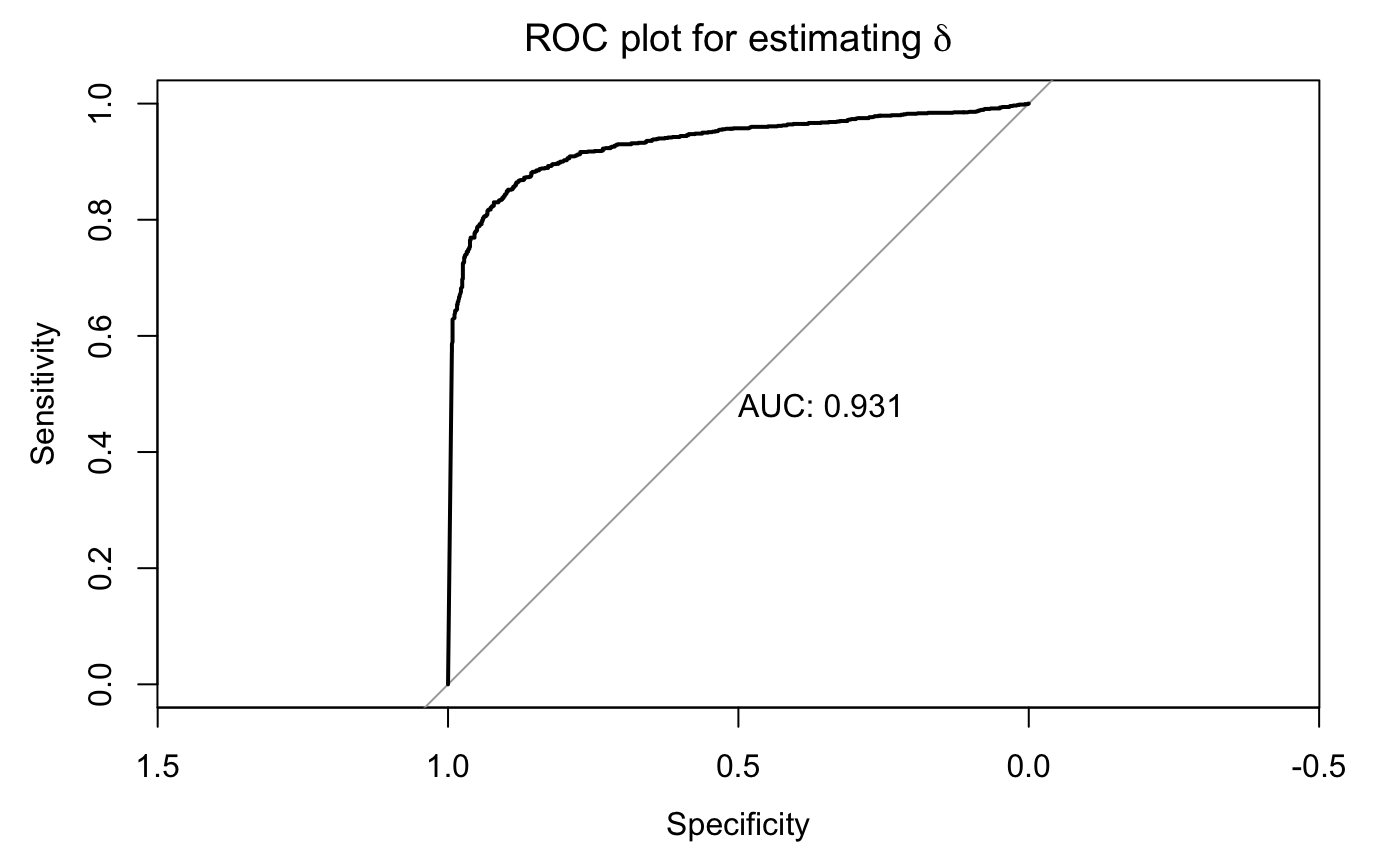

Citation

Shuang Jiang, Guanghua Xiao, Andrew Y. Koh, Qiwei Li, Xiaowei Zhan (2018), A Bayesian Zero-Inflated Negative Binomial Regression Model for the Integrative Analysis of Microbiome Data, arXiv:1812.09654. link.

Contact

Shuang Jiang shuangj@mail.smu.edu Last updated on June 6, 2019.

Integrative Bayes Model

Shuang Jiang et al

12/03/2018